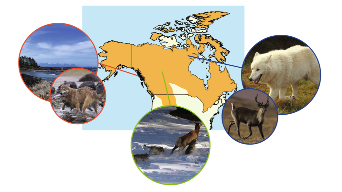
This section will focus on analyzing SNP data from North American gray wolves (Canis lupus). The original data consist of a few hundred wolf samples that were enriched for a custom capture array consisting of several thousands of regions across the wolf genome.
Our data consist of genic SNPs genotyped for three wolf ecotypes: (1) the British Columbia coastal, (2) the High Arctic, and (3) the Boreal Forest. These wolves have pretty striking ecological and behavioral differences that are in part driven by differences amongst their environments. We used these data to look at population genetic variation and signals of local adaptation amongst these ecotypes (Schweizer et al. 2015, Molecular Ecology).
This data are also included in the project repo you previously cloned. Let's navigate to the wolf-snps
folder now to minimize the paths we have to type when using the data. You should already be in the root project directory
(~/congen-bioinformatics/), so you should just have to type the command:
cd data/wolf-snps/Click to see command breakdown
| Command line parameter | Description |
|---|---|
| cd | The Linux change directory command |
| data/wolf-snps | The path to the directory you want to change to. In this case,
this is a relative path. If you are not in the ~/congen-bioinformatics/ directory,
you will likely get an error saying this path does not exist. |
If you are somewhere else other than the root project directory, first navigate back to that folder and then change to the
wolf-snps folder. Or, if you're familiar enough with the file tree, navigate straight to the
data folder!
Lost somewhere in the file system? Not sure exactly where you are? Remember the print working directory command:
pwd. This simply prints your current location in the file system and can help you get your
bearings if you've been moving around a lot. This and ls are essential for navigating your
file system.
I've downsampled the full data set to a subset of 35 individuals and a subset of genic SNPs. We will be working with these SNP data in a VCF file. VCF stands for variant call format and is a tab-delimited plain text file that stores genetic variants, such as SNPs, insertions, and deletions, found by comparing sequenced samples to a reference genome. Each site is described by its location, alleles, and quality scores, plus each individual's genotype, depth of coverage, and more, at that site. Note that sites can be both variable and non-variable.
The full VCF file format specifications can be found here: samtools VCF specs
VCF files also contain a header, denoted with the # character at the beginning of the line.
The header can be a single line or thousands of lines and provides information on how the VCF file was generated, to which reference genome
the sequence data was aligned, and definitions of what the various fields in each column of the data mean. Given all this information, VCF files
can potentially be enormous in size and cumbersome to work with.
Luckily, there is software out there to help! PLINK is a widely used
toolset for working with genotype data. It was originally developed for human genome-wide association studies, but it works with data from
any diploid organism and can read VCF files directly. PLINK can be used to filter SNPs and individuals, assess data quality such as
missingness, and calculate a variety of statistics like allele frequencies, Hardy-Weinberg equilibrium, and per-individual genotype counts.
We'll be using PLINK 2, the current version of the program, which is run with the command plink2.
Unlike many of the Unix commands we've seen so far, PLINK doesn't print its results to the terminal to be piped (|) or
redirected (>). Instead, it writes its results to files whose names start with a prefix you choose with the
--out option, and the file extension is determined by the analysis. Every run also writes a .log file that records the
command you ran and a summary of what PLINK did, which is handy for checking your work later. In general, the program is called
as follows:
plink2 <input option> <input file> <analysis options> --out <output prefix>Click to see command breakdown
| Command line parameter | Description |
|---|---|
| plink2 | A program for working with genotype data, including variant calls in VCF format |
| <input option> | The option specifying the format of the input file,
e.g. --vcf for a VCF file |
| <input file> | The path to the file you want to run on |
| <analysis options> | The analyses to run, plus any options for filtering SNPs or samples |
| --out | The option to specify the prefix for all output files |
| <output prefix> | The desired prefix for the output files. The file extension will be determined by the analysis. |
Here are some more explicit examples of PLINK commands:
# Calculate allele frequencies for every SNP (writes input_freqs.afreq)
plink2 --vcf input.vcf --dog --freq --out input_freqs

# Report the amount of missing data per sample and per SNP (writes input_missing.smiss and input_missing.vmiss)
plink2 --vcf input.vcf --dog --missing --out input_missing

# Keep only the samples listed in a file and write them to a new VCF (writes input_subset.vcf)
plink2 --vcf input.vcf --dog --keep samples.txt --export vcf --out input_subset
Because PLINK was built for human data, it assumes human chromosomes by default: 22 autosomes plus the sex chromosomes and
mitochondria. Wolves have 38 pairs of autosomes, the same as domestic dogs, so we add the --dog option to every
PLINK command. Before running PLINK on a new data set, it's a good idea to check how the chromosomes are named in the
VCF file:
grep -v "#" Filtered_NAwolf_n35_variableSites_GenicRegions.recode.vcf | cut -f1 | sort | uniq -c
Here, cut -f1 keeps only the first tab-separated column of each line, which in a VCF file is the chromosome name.
Then sort | uniq -c groups identical names together and counts how many SNPs are on each chromosome.
If the chromosomes are numbered (like 1 through 38, or chr1 through chr38),
--dog will work. If they're scaffold or contig names instead, use the --allow-extra-chr option.
For this section of the workshop, we're going to start with a simple task, calculating heterozygosity, for a single wolf ecotype. Then we're going to learn how to automate it over multiple populations through using loops and writing a script.
Before we do that, let's get some basic info about our called variants in the VCF file.
TASK 1: How many SNPs are there?
We know that our VCF file has a number of header lines (which don't count towards the actual number of SNPs) and then a separate
line for each SNP. Because of this, if we just use wc -l we will count all lines of the file, which doesn't
tell us the number of SNPs.
But by using grep with the -v flag, we can find all the lines of text that don't
contain a character, string, or pattern. Then we can use our handy | to get our answer:
grep -v "^#" Filtered_NAwolf_n35_variableSites_GenicRegions.recode.vcf | wc -lClick to see command breakdown
| Command line parameter | Description |
|---|---|
| grep | A Unix string and pattern searching command |
| -v | By default, grep prints all lines that contain
the specified string/pattern. The -v option tells grep to print
all the lines that DO NOT contain the specified string/pattern instead. |
| "#" | The string or pattern you want to search for |
| Filtered_NAwolf_n35_variableSites_GenicRegions.recode.vcf | The path to the file you want to search |
| | | The pipe character means the output from the command specified before it will be used as the input to the command specified after it |
| wc | The Linux word count command. Counts the number of lines, words, and characters in an input file. |
| -l | Tells wc to only count number of lines |
This should output the number of lines in the VCF file that don't contain the "#" character:
19620Since the only lines with "#" should be the informational header lines and all other lines represent one SNP, this means there are 19,620 SNPs represented in this VCF file.
TASK 2: Calculate heterozygosity for the coastal wolf samples.
We're going to use one of the functions of PLINK to count the homozygous and heterozygous genotypes
(--sample-counts) of each individual within only the coastal wolf population. PLINK lets us specify which individuals to
include in an analysis through the --keep option with a file of sample IDs.
plink2 --vcf Filtered_NAwolf_n35_variableSites_GenicRegions.recode.vcf --dog --keep pop_coastal.txt --sample-counts cols=hom,het --out Filtered_NAwolf_n35_variableSites_GenicRegions_coastalClick to see command breakdown
| Command line parameter | Description |
|---|---|
| plink2 | A program for working with genotype data, including variant calls in VCF format |
| --vcf | The option to specify that the input file is a VCF file |
| Filtered_NAwolf_n35_variableSites_GenicRegions.recode.vcf | The path to the input file |
| --dog | Tells PLINK to use the dog chromosome set, which wolves share. Without this, PLINK assumes human chromosomes. |
| --keep | This option is used with a file that lists sample IDs. Only samples in that file will be used by the program for this run. |
| pop_coastal.txt | The path to the file with the sample IDs to keep. |
| --sample-counts | This option tells PLINK to count the genotypes of different types (homozygous, heterozygous, missing, etc.) for each sample. |
| cols=hom,het | A modifier for --sample-counts that sets which columns
to report: here, the number of homozygous genotypes (hom) and heterozygous genotypes (het) for
each sample. Without it, PLINK reports a longer default set of columns. |
| --out | The option to specify the prefix for all output files. The file extension will be determined by the analysis. |
| Filtered_NAwolf_n35_variableSites_GenicRegions_coastal | The desired name of the output file. If it exists it will be overwritten. |
Every time PLINK runs, it writes a .log file. The log records the exact command you ran, how many samples and
variants PLINK loaded, how many remained after filtering, and any warnings. Make a habit of reading it after every run:
cat Filtered_NAwolf_n35_variableSites_GenicRegions_coastal.log
Find the lines reporting how many samples were loaded and how many remained after --keep. Does the number
remaining match the number of IDs in the pop file?
wc -l pop_coastal.txtTry this: Make a copy of the pop file with a typo in one sample ID, then rerun PLINK with the copy. Does PLINK stop with an error? Does it tell you anything in the terminal or the log? If a problem like this doesn't cause an error, the log may be the only place you'd notice it.
sed '1s/.$/X/' pop_coastal.txt > pop_coastal_typo.txtplink2 --vcf Filtered_NAwolf_n35_variableSites_GenicRegions.recode.vcf --dog --keep pop_coastal_typo.txt --sample-counts cols=hom,het --out typo_test
If we use ls to look at the output files, we can see that PLINK has provided a .log file, which contains our command and a
summary of the run, as well as a .scount file that provides the per-individual genotype counts.
But does this file actually give us the heterozygosity?
head Filtered_NAwolf_n35_variableSites_GenicRegions_coastal.scountClick to see command breakdown
| Command line parameter | Description |
|---|---|
| head | A Unix command that prints the first few lines of a file |
| Filtered_NAwolf_n35_variableSites_GenicRegions_coastal.scount | The path to the input file |
No, the output provides the number of homozygous genotypes and the number of heterozygous genotypes for each individual, below a
header line that starts with #IID. But we can use this information with a handy one-liner in awk to calculate
heterozygosity, the proportion of each individual's genotyped sites that are heterozygous:
awk 'NR > 1 {print $1, $2, $3, $3/($2+$3)}' Filtered_NAwolf_n35_variableSites_GenicRegions_coastal.scount > Filtered_NAwolf_n35_variableSites_GenicRegions_coastal.scount.calcClick to see command breakdown
| Command line parameter | Description |
|---|---|
| awk | A Linux text processing language |
| 'NR > 1 {print $1, $2, $3, $3/($2+$3)}' |
The user-coded program to run. NR is awk's built-in count of the current line number, so
NR > 1 skips the header line. For every other line, this prints the sample ID ($1), the
homozygous count ($2), the heterozygous count ($3), and the heterozygosity: the heterozygous
count divided by the number of sites where this sample had a genotype call — homozygous plus
heterozygous, so missing genotypes are excluded. |
| Filtered_NAwolf_n35_variableSites_GenicRegions_coastal.scount | The path to the file on which to run the program |
| > | The redirect character means the output from the command specified before it will be saved to the file specified after it |
| Filtered_NAwolf_n35_variableSites_GenicRegions_coastal.scount.calc | The path to the desired output file. This will be created if it doesn't exist and WILL OVERWRITE files that do exist |
One thing to be clear about before we go further: the denominator here is the number of SNPs in this file that the individual was genotyped at, not the number of bases in the wolf genome. Our VCF only contains sites that were variable somewhere in the full data set, so what we're calculating is the proportion of those SNPs at which an individual is heterozygous. That's a good number for comparing individuals and populations to each other here, because every sample is measured against the same set of sites. But it isn't genome-wide heterozygosity, which is reported per base pair and is a far smaller number. Calculating that would also require the invariant sites, plus a record of which positions had enough coverage to be called at all.
Each step of our analysis should keep one line per individual, so a quick line count can catch samples that were silently dropped along the way:
wc -l pop_coastal.txt Filtered_NAwolf_n35_variableSites_GenicRegions_coastal.scount Filtered_NAwolf_n35_variableSites_GenicRegions_coastal.scount.calc
The .scount file should have one more line than the pop file (for its header line), and the
.scount.calc file should have the same number of lines as the pop file. If the numbers don't line up,
something in the pipeline removed or added lines, and you'll want to find out what before using the results.
This kind of check matters because filtering steps can remove data without any error. For example, an earlier version
of this tutorial used the awk pattern /RKW/ to select sample lines. Any wolf whose ID didn't contain
"RKW" would have vanished from the results without a single warning. Only counting lines would have caught it.
Counting lines tells you whether the number of samples is right, but not whether they're the right samples. Let's check that the sample IDs in our results exactly match the IDs in the pop file. First, save a sorted copy of each list of IDs:
sort pop_coastal.txt > pop_coastal_ids.txtawk '{print $1}' Filtered_NAwolf_n35_variableSites_GenicRegions_coastal.scount.calc | sort > calc_coastal_ids.txt
Then compare the two lists with diff, which prints any lines that differ between two files:
diff pop_coastal_ids.txt calc_coastal_ids.txtClick to see command breakdown
| Command line parameter | Description |
|---|---|
| diff | A Unix command that compares two files line by line and prints the lines that differ |
| pop_coastal_ids.txt | The first file to compare. Lines only in
this file are printed with a < in front. |
| calc_coastal_ids.txt | The second file to compare. Lines only in
this file are printed with a > in front. |
If diff prints nothing, the lists are identical. If it does print something, those are samples that were
dropped, added, or renamed along the way. Differences can also come from invisible characters, like trailing spaces
or Windows-style line endings in a pop file, which is worth knowing because they can also make PLINK fail to match
sample IDs.
Software can have bugs, and more often, it can calculate something slightly different from what you assumed. One of
the best ways to check a result is to recompute it yourself for a single sample. Pick one coastal wolf (the first ID
in head -1 pop_coastal.txt works), and replace SAMPLE_ID below with that ID.
First, find which column of the VCF file holds that sample's genotypes. The line starting with #CHROM contains
the column names, so we split it into one name per line and find the line number of our sample:
grep "^#CHROM" Filtered_NAwolf_n35_variableSites_GenicRegions.recode.vcf | tr '\t' '\n' | grep -n -x "SAMPLE_ID"Click to see command breakdown
| Command line parameter | Description |
|---|---|
| grep "^#CHROM" | Finds the line that starts with #CHROM.
The ^ means "at the start of the line," so this matches only the column-name line, not other
header lines that contain the text elsewhere. |
| tr '\t' '\n' | The Unix translate command. Replaces every tab with a newline, so each column name ends up on its own line. |
| grep -n | The -n option tells grep to print the
line number of each match in front of it, followed by a :. Since each column name is now on
its own line, the line number is the column number. |
| -x | Tells grep to match only lines that are
exactly the search text, rather than lines that contain it. Without -x,
searching for a sample like RKW1 would also match RKW10, RKW11, and so on. |
| "SAMPLE_ID" | The sample ID to search for |
The number before the : is the column number. Now pull out that column for every SNP, keep just the genotype
(the first :-separated field), and count each genotype type, replacing COLUMN with that number:
grep -v "^#" Filtered_NAwolf_n35_variableSites_GenicRegions.recode.vcf | cut -f COLUMN | cut -d: -f1 | sort | uniq -cClick to see command breakdown
| Command line parameter | Description |
|---|---|
| grep -v "^#" | Prints every line that does not start
with #, which removes the header and keeps one line per SNP |
| cut -f COLUMN | The Unix cut command, which pulls out selected
columns (fields) from each line. By default, cut splits lines at tabs, so -f followed
by a number keeps just that tab-separated column: here, our sample's column. |
| cut -d: -f1 | Each sample's entry looks like 0/1:12:99,
with the genotype first and other information (like read depth and quality) after it, separated by
colons. The -d: option tells cut to split at : instead of tabs, and
-f1 keeps only the first piece: the genotype. |
| sort | Sorts the genotypes so identical ones are next to each other |
| uniq -c | Collapses identical adjacent lines into one and, with
-c, counts how many times each appeared. uniq only merges lines that are next to each
other, which is why we sort first. |
You should see counts for genotypes like 0/0 and 1/1 (homozygous), 0/1 (heterozygous), and
possibly ./. (missing). Use these counts to calculate heterozygosity yourself: the number of heterozygous
genotypes divided by the number of homozygous plus heterozygous genotypes. Then compare your answer to PLINK's:
grep "SAMPLE_ID" Filtered_NAwolf_n35_variableSites_GenicRegions_coastal.scount.calc
Do they match? If not, why not? Look closely at the genotype codes you counted. Did you see any written with
| instead of /, or any other codes you didn't expect?
Using this, we can also calculate the mean population heterozygosity using awk:
awk '{sum += $4} END {if (NR > 0) print sum / NR }' Filtered_NAwolf_n35_variableSites_GenicRegions_coastal.scount.calcClick to see command breakdown
| Command line parameter | Description |
|---|---|
| awk | A Linux text processing language |
| '{sum += $4} END {if (NR > 0) print sum / NR }' |
The user-coded program to run. This adds up the heterozygosity values in column 4, then divides the total by the
number of lines (NR) to get the mean. |
| Filtered_NAwolf_n35_variableSites_GenicRegions_coastal.scount.calc | The path to the file on which to run the program |
Before trusting a result, ask whether it's even possible. Heterozygosity is a proportion, so every value must be between 0 and 1. Sorting the results by heterozygosity (column 4) puts the extremes at the top and bottom, where problems are easiest to spot:
sort -k4,4n Filtered_NAwolf_n35_variableSites_GenicRegions_coastal.scount.calcClick to see command breakdown
| Command line parameter | Description |
|---|---|
| sort | The Unix command to sort lines of text |
| -k4,4 | Sort using only column 4 |
| n | Sort numerically rather than alphabetically |
Are any values outside 0 to 1? Is any individual far from the rest? An outlier isn't necessarily wrong, but it's worth investigating. For example, check whether that individual has many more missing genotypes than the others.
Try this: Sometimes code runs without errors and gives numbers that look reasonable, but it's calculating the
wrong thing. Run this version of our awk command and look at the results:
awk 'NR > 1 {print $1, $2, $3, $2/($2+$3)}' Filtered_NAwolf_n35_variableSites_GenicRegions_coastal.scountAll the values are between 0 and 1, and nothing crashes. What did this command actually calculate? Compare these values with the heterozygosity values you calculated above. Would you have caught the mistake if you didn't already know roughly what to expect?
Great! So now we have calculated the per-individual heterozygosity and the population heterozygosity for the coastal populations. Let's figure out how to repeat this set of commands for any number of additional populations.
Instead of hard-coding our command to be specific to the coastal wolves, we can use shell variables. We indicate a shell variable like so:
wolf_pop=coastalClick to see command breakdown
| Command line parameter | Description |
|---|---|
| wolf_pop | The desired variable name appears to the left of the equals sign |
| = | The equals sign indicates variable assignment in programming languages |
| coastal | The value you wish to assign to the variable name |
We can check that variable assignment was successful by printing the value with the echo command:
echo ${wolf_pop}Click to see command breakdown
| Command line parameter | Description |
|---|---|
| echo | The Unix print command. Values given as input will be printed to the screen. |
| ${wolf_pop} | The item to print to the screen. In this case, because wolf_pop is a
defined variable, we must use the ${} symbols to let echo know to print its assigned value to the screen, rather
than just the text "wolf_pop". |
We can use variables in any command in the terminal. For instance, we can run the same command as before to count genotypes, but instead of typing "coastal" in the command, we can use our variable:
plink2 --vcf Filtered_NAwolf_n35_variableSites_GenicRegions.recode.vcf --dog --keep pop_${wolf_pop}.txt --sample-counts cols=hom,het --out Filtered_NAwolf_n35_variableSites_GenicRegions_${wolf_pop}Click to see command breakdown
| Command line parameter | Description |
|---|---|
| plink2 | A program for working with genotype data, including variant calls in VCF format |
| --vcf | The option to specify that the input file is a VCF file |
| Filtered_NAwolf_n35_variableSites_GenicRegions.recode.vcf | The path to the input file |
| --dog | Tells PLINK to use the dog chromosome set, which wolves share. Without this, PLINK assumes human chromosomes. |
| --keep | This option is used with a file that lists sample IDs. Only samples in that file will be used by the program for this run. |
| pop_${wolf_pop}.txt | The path to the file with the sample IDs to keep. In
this case, we're using our variable, wolf_pop, to indicate which existing population file to use. |
| --sample-counts | This option tells PLINK to count the genotypes of different types (homozygous, heterozygous, missing, etc.) for each sample. |
| cols=hom,het | A modifier for --sample-counts that sets which columns to
report: here, the number of homozygous genotypes (hom) and heterozygous genotypes (het) for each
sample. Without it, PLINK reports a longer default set of columns. |
| --out | The option to specify the prefix for all output files. The file extension will be determined by the analysis. |
| Filtered_NAwolf_n35_variableSites_GenicRegions_${wolf_pop} |
The desired name of the output file. If it exists it will be overwritten. In this case, we use the wolf_pop
variable to create a file with the name of the current population. |
This provides the same output as the command we ran earlier. So, we could assign a new value to the wolf_pop
variable. Notice also how I have been consistent in how I named all of my pop files so that I can substitute an ecotype
name but otherwise still have that same general file name structure.
wolf_pop=highArcticClick to see command breakdown
| Command line parameter | Description |
|---|---|
| wolf_pop | The desired variable name appears to the left of the equals sign |
| = | The equals sign indicates variable assignment in programming languages |
| highArctic | The value you wish to assign to the variable name |
We can check that variable assignment was successful by printing the value with the echo command:
echo ${wolf_pop}Click to see command breakdown
| Command line parameter | Description |
|---|---|
| echo | The Unix print command. Values given as input will be printed to the screen. |
| ${wolf_pop} | The item to print to the screen. In this case, because wolf_pop is a
defined variable, we must use the ${} symbols to let echo know to print its assigned value to the screen, rather
than just the text "wolf_pop". |
Now that we've reassigned the wolf_pop variable to the highArctic population, we can run the same series of commands as above,
but PLINK will use the samples and provide output for this population.
First, run PLINK to count the homozygous and heterozygous genotypes:
plink2 --vcf Filtered_NAwolf_n35_variableSites_GenicRegions.recode.vcf --dog --keep pop_${wolf_pop}.txt --sample-counts cols=hom,het --out Filtered_NAwolf_n35_variableSites_GenicRegions_${wolf_pop}Click to see command breakdown
| Command line parameter | Description |
|---|---|
| plink2 | A program for working with genotype data, including variant calls in VCF format |
| --vcf | The option to specify that the input file is a VCF file |
| Filtered_NAwolf_n35_variableSites_GenicRegions.recode.vcf | The path to the input file |
| --dog | Tells PLINK to use the dog chromosome set, which wolves share. Without this, PLINK assumes human chromosomes. |
| --keep | This option is used with a file that lists sample IDs. Only samples in that file will be used by the program for this run. |
| pop_${wolf_pop}.txt | The path to the file with the sample IDs to keep. In
this case, we're using our variable, wolf_pop, to indicate which existing population file to use. |
| --sample-counts | This option tells PLINK to count the genotypes of different types (homozygous, heterozygous, missing, etc.) for each sample. |
| cols=hom,het | A modifier for --sample-counts that sets which columns to
report: here, the number of homozygous genotypes (hom) and heterozygous genotypes (het) for each
sample. Without it, PLINK reports a longer default set of columns. |
| --out | The option to specify the prefix for all output files. The file extension will be determined by the analysis. |
| Filtered_NAwolf_n35_variableSites_GenicRegions_${wolf_pop} |
The desired name of the output file. If it exists it will be overwritten. In this case, we use the wolf_pop
variable to create a file with the name of the current population. |
Then run awk to calculate heterozygosity for each individual in the highArctic sample. Again note that we use the
wolf_pop variable in our input and output file names:
awk 'NR > 1 {print $1, $2, $3, $3/($2+$3)}' Filtered_NAwolf_n35_variableSites_GenicRegions_${wolf_pop}.scount > Filtered_NAwolf_n35_variableSites_GenicRegions_${wolf_pop}.scount.calcClick to see command breakdown
| Command line parameter | Description |
|---|---|
| awk | A Linux text processing language |
| 'NR > 1 {print $1, $2, $3, $3/($2+$3)}' | The user-coded program to run |
| Filtered_NAwolf_n35_variableSites_GenicRegions_${wolf_pop}.scount |
The path to the file on which to run the program. Note that we use the wolf_pop variable to indicate
the population file to run. |
| > | The redirect character means the output from the command specified before it will be saved to the file specified after it |
| Filtered_NAwolf_n35_variableSites_GenicRegions_${wolf_pop}.scount.calc |
The path to the desired output file. This will be created if it doesn't exist and WILL OVERWRITE files that do exist.
Note that we use the wolf_pop variable to save to a file name labeled with the correct population. |
And then awk again with the wolf_pop variable to get mean population heterozygosity:
awk '{sum += $4} END {if (NR > 0) print sum / NR }' Filtered_NAwolf_n35_variableSites_GenicRegions_${wolf_pop}.scount.calcClick to see command breakdown
| Command line parameter | Description |
|---|---|
| awk | A Linux text processing language |
| '{sum += $4} END {if (NR > 0) print sum / NR }' | The user-coded program to run |
| Filtered_NAwolf_n35_variableSites_GenicRegions_${wolf_pop}.scount.calc |
The path to the file on which to run the program. Note that we use the wolf_pop variable to indicate
the population file to run. |
Now, we're going to add some of these commands with variables to a script so that we can automate the series of commands to generate per-individual and per-population heterozygosity.
A script is simply a text file where we can write and save the code and commands we want to run. Scripts give us the flexibility to perform complex operations based on conditions and ranges of values. Since a script is a text file, we're going to create a new text file and copy some commands into it. We're going to use an in-terminal text editor, vim, to do this, although there are several other options.
vim het_analysis.shClick to see command breakdown
| Command line parameter | Description |
|---|---|
| vim | An in-terminal text editor available on Linux. |
| het_analysis.sh | The name of the text file to create or view (if it exists). The .sh extension indicates this is a shell script |
You should now be in the vim text editor. Your screen should be cleared of commands and the cursor should be blinking on top, with
tilde characters (~) on every other line. Importantly, vim has both a viewing mode and an editing mode.
When you create a new file with vim, as we have here, you start out in viewing mode. We can switch to editing mode
by pressing the a key. Once you do this, you'll see the text -- INSERT -- at the bottom of the screen, indicating we have
switched to editing mode.
Now, we can copy and paste our commands for calculating heterozygosity into this file. Of course, there are other ways we could get the
commands into the file (such as using echo and redirecting), but we'll stay simple today.
Copy the following commands:
wolf_pop=$1
plink2 --vcf Filtered_NAwolf_n35_variableSites_GenicRegions.recode.vcf --dog --keep pop_${wolf_pop}.txt --sample-counts cols=hom,het --out Filtered_NAwolf_n35_variableSites_GenicRegions_${wolf_pop}
awk 'NR > 1 {print $1, $2, $3, $3/($2+$3)}' Filtered_NAwolf_n35_variableSites_GenicRegions_${wolf_pop}.scount > Filtered_NAwolf_n35_variableSites_GenicRegions_${wolf_pop}.scount.calc
awk '{sum += $4} END {if (NR > 0) print sum / NR }' Filtered_NAwolf_n35_variableSites_GenicRegions_${wolf_pop}.scount.calc
The last three commands should be familiar to you already. They are the same commands we used above for the coastal population, but
we've substituted the string "coastal" for the variable wolf_pop.
The first line, wolf_pop=$1, is our variable assignment. It tells the script to assign the variable wolf_pop the value
of $1. Well what is $1? It has a dollar sign ($) preceding it, so we know it is a variable. But we haven't
assigned anything to it yet.
Like other commands, your own scripts can take input options from the command line. By default, a shell script (like the one we are
writing) will assign these options to internal variables: $1 for the first option, $2 for the second one, and so on.
So, wolf_pop will be assigned whatever we type into the terminal when we run the script.
Let's exit out of vim to try and run our script. First, switch back to viewing mode by pressing the ESC key.
You should no longer see the text -- INSERT -- at the bottom of the screen. When in viewing mode, any input we type
is interpreted as internal vim commands, such as saving, exiting, etc. Let's tell vim to save the changes we've made to
the file with the write command (w) and then quit (q) the text editor by typing:
:wqClick to see command breakdown
| Command line parameter | Description |
|---|---|
| : | Tells vim to interpret the following text as commands |
| w | The vim write command that saves changes made to the file |
| q | The vim quit command to exit the text editor and return to the
terminal |
TASK 3: Make the script executable and try it
We will use the chmod command to change the permissions on the script so the shell knows that its contents
should be interpreted as commands. This is known as making the file executable:
chmod a+x het_analysis.shClick to see command breakdown
| Command line parameter | Description |
|---|---|
| chmod | The Unix change mode command used to change permissions on files |
| a+x | This tells chmod to give all users (a) permission to
execute the file (+x) |
| het_analysis.sh | The name of the file to change permissions |
Now let's try to execute our file on the coastal population:
./het_analysis.sh coastalClick to see command breakdown
| Command line parameter | Description |
|---|---|
| ./het_analysis.sh | The name of the file to run. Since we have changed its
permissions to be executable, its contents will be interpreted as shell commands. ./ also indicates to
run this file as a shell script |
| coastal | Remember, the script we wrote expects input from the command
line to assign to the $1 variable. This will be that value |
If we use our handy ls -lht command, we can see that the three newest files are of the coastal wolf samples, and that
the script we wrote printed the mean population heterozygosity to the screen.
Software changes over time. New versions can change default settings, rename options, or reorder output columns, which can change your results without any error. To make sure you (or anyone else) can reproduce your analysis later, record which version of each program you used:
plink2 --version
You can also add this line to the top of het_analysis.sh, so every run of the script records the version it
used alongside its output.
A few other habits help here:
- Keep your
.logfiles. They record exactly what PLINK did on each run. - Run every step from a script. Avoid editing output files by hand. A script is a complete record of how you got from raw data to results, and you can rerun it after fixing a mistake.
- Rerun the whole script when something changes. If you fix a pop file or change a command, rerun the script from the beginning instead of patching individual outputs. This keeps every result consistent with the current inputs.
Documenting our code with comments and print statements
It is also good practice to document what each step of our code does in human-readable language. This is called commenting
our code. The way to comment code differs between programming languages, but a fairly common method (used in Python, R, and the shell
scripting we're doing) is with the # symbol. For languages that use this symbol, any line starting with # will
be interpreted as a comment rather than a command to be run.
We can also provide some helpful context to the output of our script. Rather than just printing out a number that may be confusing
to someone else using the script (or even ourselves if we re-run this same script months or years later), we can use echo
within the script to print some more information, like that the number printed represents mean population heterozygosity.
Feel free to open up your script and follow along as I comment my version and add contextual print statements:
vim het_analysis.shClick to see command breakdown
| Command line parameter | Description |
|---|---|
| vim | An in-terminal text editor available on Linux. |
| het_analysis.sh | The name of the text file to create or view (if it exists). The .sh extension indicates this is a shell script |
TASK 4: Which population has the highest mean heterozygosity?
To find this out now, all we have to do is run our script on all three populations:
./het_analysis.sh coastal
./het_analysis.sh highArctic
./het_analysis.sh borealForest
This shows that the boreal forest population has the highest mean heterozygosity at 0.190026. Remember what that number is: the average proportion of our panel of SNPs at which an individual is heterozygous. It's the right number for ranking these three ecotypes against each other, but not comparable to heterozygosity values you'd read in a paper.
for loops
If only there was a way to automate the analysis even further... Aha! We can use for loops to call the script
multiple times with different input values, in this case our 3 population strings, for the wolf_pop variable.
for loops in a shell script are generated in a similar way as in other programming languages:
for <variable> in <iterable>; do <code>; doneClick to see command breakdown
| Command line parameter | Description |
|---|---|
| for | The start of the for loop |
| <variable> | for loops iterate over a set of values. Whatever
is named here as <variable> will be the variable name of the current value in the set. |
| in | Indicates that the following will be the set of values to iterate over |
| <iterable>; | A data type that contains multiple values |
| do | A keyword that indicates a block of code within a for loop
has started |
| <code>; | The code to execute on each value in the set of values |
| done | A keyword that indicates the end of the for loop |
For instance, we could do the following to loop over letters in the alphabet from A to F and print them out:
for letter in {A..F}; do echo $letter; doneOr the following to subtract 1 from each integer from 1 to 4 and print the resulting value to the screen:
for num in 1 2 3 4; do echo "The value of $num - 1 is " `expr $num - 1`; doneTASK 5: Use a for loop to calculate heterozygosity for the three wolf ecotypes
for pop in coastal highArctic borealForest; do ./het_analysis.sh $pop; doneClick to see command breakdown
| Command line parameter | Description |
|---|---|
| for | The start of the for loop |
| pop | This tells the for loop to assign the current value
being executed to the $pop variable |
| in | Indicates that the following will be the set of values to iterate over |
| coastal highArctic borealForest | The values over which to iterate |
| do | A keyword that indicates a block of code within a for loop
has started |
| ./het_analysis.sh $pop; | Run the het_analysis.sh script on the current
value stored in $pop |
| done | A keyword that indicates the end of the for loop |
This should produce the same output as when we ran the three commands manually above!
Hopefully you've become more familiar with how to use variables in the command-line and in scripts, how to write a script and edit it
using vim, and how to use for loops to make your life easier!